Predictive Maintenance Software: How It Actually Works

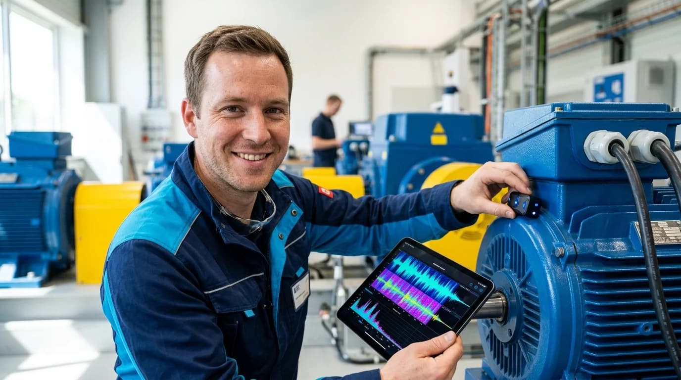
Predictive maintenance software is an industrial analytics and execution system that continuously monitors the physical health of production machinery (via vibration spectra, motor current signatures, acoustics, thermography, and lubricant condition) to detect nascent component degradation and schedule repairs inside planned downtime windows before a breakdown happens. Rather than servicing machines on arbitrary calendar intervals or waiting for a spindle to seize mid-shift, predictive maintenance (PdM) software models where each critical asset sits on its degradation curve and triggers a parts-ready work order in the maintenance system weeks ahead of functional failure.

Most vendor brochures portray predictive maintenance as a magic artificial intelligence black box that ingests raw sensor numbers and predicts exact failure dates on day one. Practitioners who have wired accelerometers to 20-year-old stamping presses know the engineering reality is far more concrete. Without operating context from the PLC (spindle RPM, load torque, active product recipe), a machine learning model mistakes a heavy roughing cut for a failing bearing. Below is the engineering blueprint for how predictive maintenance software actually works: the ISO 13374 six-stage processing pipeline, sensor physics across the P-F curve, edge Digital Signal Processing (DSP) and Fast Fourier Transform (FFT) bearing kinematics, Remaining Useful Life (RUL) modeling when failure labels are scarce, and closed-loop integration with your CMMS software and MES.

The short version

• ISO 13374 six-stage architecture: Production PdM software follows ISO 13374 from high-frequency Data Acquisition and Edge DSP Manipulation through State Detection, Health Assessment, Prognostics (RUL), and automated CMMS Advisory Generation.
• P-F curve physics dictate modality: Ultrasonic demodulation and FFT envelope vibration catch bearing race spalling 4 to 12 weeks before failure, motor current signature analysis (MCSA) catches rotor bar and coupling faults in the cabinet, and thermal rise confirms late-stage friction.
• Edge DSP beats raw cloud streaming: Sampling a tri-axial accelerometer at 25.6 kHz generates \sim 20 GB/day per sensor; edge gateways compute velocity RMS, kurtosis, crest factor, and bearing fault frequencies (BPFO, BPFI, BSF, FTF) locally, streaming compact feature vectors over MQTT Sparkplug B.
• Context-conditioned anomaly detection first: Because confirmed run-to-failure histories are rare in a single plant, deployments start with ISO 20816 vibration limits and recipe-conditioned anomaly models trained on healthy runs, evolving to Weibull and survival/RUL models as teardown labels accumulate.
• Zero-fatigue CMMS automation: Joining condition telemetry with PLC states over OPC UA suppresses false alarms during cold starts and changeovers, issuing one idempotent CMMS work order with the suspect component and reserved spare part.
• Targeted asset ROI: Instrumenting the 10% to 20% of bottleneck assets whose breakdowns halt the line delivers measurable OEE Availability gains within one to two quarters.

The ISO 13374 six-stage predictive maintenance software architecture

To prevent condition monitoring tools from turning into isolated data silos, ISO 13374 (Condition monitoring and diagnostics of machines) and the MIMOSA Open Systems Architecture for Enterprise Application Integration (OSA-EAI) standardize predictive maintenance software into six sequential functional blocks.

1. Block 1: Data Acquisition (DA): Converts physical machine phenomena (housing acceleration, magnetic flux, acoustic pressure, infrared radiation) into calibrated digital time-series waveforms stamped with IEEE 1588 PTP UTC time and asset topology IDs.
2. Block 2: Data Manipulation (DM) / Signal Processing: Executes anti-aliasing filtration, Hanning windowing, high-frequency envelope demodulation, Fast Fourier Transforms (FFT), and time-domain statistical compression (RMS, Peak-to-Peak, Kurtosis, Crest Factor) on the edge IPC or smart sensor gateway.
3. Block 3: State Detection (SD): Joins the extracted spectral features with real-time operational context from the PLC (Spindle_RPM, Motor_Load_Pct, Active_Recipe_ID, PackML_State) and evaluates whether the asset is within its normal operating envelope.
4. Block 4: Health Assessment (HA) / Diagnostics: Classifies the specific fault mechanism and severity grade per ISO 18436-2 vibration diagnostics: distinguishing shaft unbalance (1\timesRPM) from angular misalignment (2\timesRPM axial) or an inner-race bearing spall (BPFI sidebands).
5. Block 5: Prognostics Assessment (PA): Projects the degradation trajectory forward under planned production loads from production planning software to estimate Remaining Useful Life (RUL) with confidence intervals (e.g., 180 ± 35 operating hours to critical ISO 20816 Zone D boundary).
6. Block 6: Advisory Generation (AG): Translates the prognostic window into an executable maintenance action: checking spare-part inventory in manufacturing inventory software, creating a prioritized work order in the CMMS, and recommending a repair window before the next scheduled campaign.

Matching maintenance strategy to asset criticality: RCM, SAE JA1011, and the P-F curve

No factory should put $1,500 tri-axial piezoelectric accelerometers and RUL models on an exhaust fan that costs $180 and takes 20 minutes to swap. Under SAE JA1011 (Evaluation Criteria for Reliability-Centered Maintenance Processes) and ISO 17359, maintenance engineering starts by segmenting the asset registry by Failure Effect Criticality and Failure Mode Physics.

According to reliability studies referenced in the U.S. Department of Energy (DOE) Operations & Maintenance Best Practices Guide, only 11% to 18% of industrial equipment failure modes follow a classic age-related "bathtub curve" wear-out pattern (such as refractory lining erosion, filter clogging, or sacrificial anode depletion) where fixed-interval calendar Preventive Maintenance (PM) works well. The remaining 82% to 89% of failures exhibit random or infant-mortality hazard rates where opening a healthy gearbox on a 6-month calendar schedule actually increases failure probability by introducing seal damage, contamination, or bolt-torque errors.

The P-F interval: why early detection buys weeks of scheduling lead time

Instead of calendar age, predictive maintenance exploits the P-F curve. Once a physical stress initiates a subsurface micro-crack at Point P (Potential Failure), the defect progresses through distinct physical stages before reaching Point F (Functional Failure):

Ultrasonic Stress Waves (Weeks 8-12) -> High-Freq Envelope Vibration (Weeks 4-8) -> Velocity RMS Vibration (Weeks 1-3) -> Audible Noise & Heat (Hours-Days)

The Net P-F Interval (T_PF - T_response) must be longer than the sum of spare-part procurement lead time and the time until the next planned production stop. If a specialty spindle bearing has a 3-week supplier lead time, a thermal sensor that only flags the bearing 6 hours before seizure is an emergency shutdown switch, not predictive maintenance; you need high-frequency envelope vibration or ultrasound that detects the spall 6 weeks out.

Aviation maintenance operates under strict regulatory airworthiness directives for these same prognostic models; see our companion breakdown on predictive maintenance for aircraft for how aerospace MROs validate RUL algorithms.

Sensor modalities and bearing fault physics: what the software actually measures

To diagnose which component inside a machine is failing (so the technician brings the right bearing or coupling to the line), predictive maintenance software relies on five primary sensor modalities and deterministic mechanical kinematics.

1. Tri-axial vibration and bearing fault frequency kinematics (BPFO, BPFI, BSF, FTF)

Vibration analysis is the workhorse of rotating machinery diagnostics. Every rolling-element bearing has four characteristic fault frequencies determined by shaft rotational speed (f_r, in Hz or RPM ÷ 60), number of rolling balls or rollers (N_b), rolling element diameter (d), pitch diameter (D), and contact angle (θ):

• Ball Pass Frequency Outer Race (BPFO):

BPFO = (N_b) / (2) f_r (1 - (d) / (D)cosθ\right)

- **Ball Pass Frequency Inner Race (BPFI):**
  ```text
BPFI = (N_b) / (2) f_r (1 + (d) / (D)cosθ\right)

• Ball Spin Frequency (BSF):

BSF = (D) / (2d) f_r [1 - ((d) / (D)cosθ\right)^2]

- **Fundamental Train / Cage Frequency (FTF):**
  ```text
FTF = (1) / (2) f_r (1 - (d) / (D)cosθ\right)

When a microscopic pit forms on the outer race of an SKF or Timken spindle bearing, every ball rolling over that pit produces a brief high-frequency metallic impact ring (typically between 2 kHz and 20 kHz) repeating at exactly BPFO Hz. Standard low-frequency velocity RMS (10 Hz to 1,000 Hz, governed by ISO 20816-1 / ISO 20816-3) barely budges during early spalling because the impact energy is tiny compared to overall machine vibration.

To catch the fault 8 weeks early, the software executes High-Frequency Envelope Demodulation (PeakVue / gSE): bandpass-filtering the raw acceleration waveform around the bearing's structural resonance (5 kHz to 15 kHz), rectifying the signal via a Hilbert transform to extract the impact envelope, and running an FFT on that envelope. When a sharp spectral peak emerges at BPFO and its harmonics (2\timesBPFO, 3\timesBPFO), the software names the exact bearing race weeks before temperature or overall velocity rises.

2. Motor Current Signature Analysis (MCSA)

Mounting accelerometers inside a submerged pump, a sealed hermetic compressor, or a high-temp furnace fan is physically difficult. Motor Current Signature Analysis (MCSA) clamps Hall-effect or Rogowski current transformers (CTs) safely inside the Motor Control Center (MCC) electrical cabinet.

• Broken rotor bars and end-ring cracks modulate the stator current at slip-frequency sidebands around the 50/60 Hz line frequency:

f_rotor_bar = f_line (1 ± 2 k s)

  where s is motor slip and k = 1, 2, 3\dots
- **Stator winding turn-to-turn shorts**, phase unbalance, and gearbox torque oscillations also imprint distinct sidebands in the current spectrum, making MCSA the lowest-friction retrofit for electric drive trains.

### 3. Ultrasonic acoustic emission (20 kHz to 100 kHz)

Airborne and structure-borne ultrasound sensors listen around 30 kHz to 40 kHz. In bearings, ultrasound detects early lubrication film breakdown and boundary friction before micro-spalling even begins (allowing automated grease dispensers to inject exact gram shots without over-greasing and blowing the seal). Across the wider plant, ultrasonic sensors detect compressed-air, steam-trap, and vacuum leaks that waste 20% to 30% of compressor electricity.

### 4. Infrared thermography and RTD temperature profiling

Resistance Temperature Detectors (PT100 RTDs), thermocouples, and fixed radiometric LWIR thermal cameras track heat dissipation. On mechanical bearings, a 15°C housing temperature rise sits late on the P-F curve (Stage 3/4 warning). On electrical switchgear, busbars, VFD cabinets, and induction sealing heads, however, continuous thermal imaging catches high-resistance loose lugs and failing contactors weeks before an arc flash or breaker trip.

### 5. Online oil dielectric, viscosity, and ferrous particle counters

For heavy hydraulic stamping presses, injection molding machines, and large reduction gearboxes, inline lubricant sensors measure kinematic viscosity, relative moisture saturation (% water-in-oil), dielectric constant (oxidation), and inductive ferrous/non-ferrous wear-debris particle counts per [ISO 4406 cleanliness codes](https://www.iso.org/standard/69120.html).

| Sensor Modality | Physical Measurement & Bandwidth | Primary Fault Modes Detected | Earliest P-F Detection Horizon | Typical Retrofit Hardware |
|---|---|---|---|---|
| **Piezo / MEMS Accelerometer** | Tri-axial acceleration (0.5 Hz to 10-25 kHz) | Bearing spalls (`BPFO`/`BPFI`), unbalance, misalignment, gear mesh, looseness | **4 to 12 weeks** (via envelope FFT) | Stud-mounted IEPE piezo or wireless MEMS sensor |
| **Ultrasonic Acoustic** | High-frequency stress waves (20 kHz to 100 kHz) | Lubrication starvation, micro-fretting, compressed air/vacuum valve leaks | **8 to 16 weeks** (earliest bearing stage) | Contact piezo transducer or acoustic array |
| **Motor Current (MCSA)** | 3-phase stator current & voltage (1 kHz to 10 kHz) | Broken rotor bars, air-gap eccentricity, VFD harmonics, pump cavitation | **3 to 10 weeks** | Split-core current clamps inside MCC cabinet |
| **Radiometric Thermal / RTD** | Surface IR emission or contact PT100 (1 Hz) | Loose electrical terminations, blocked cooling jackets, late bearing seizure | **Days to 6 weeks** (early for electrical; late for bearings) | Fixed LWIR PoE camera, IO-Link RTD probe |
| **Inline Oil Debris & Quality** | Ferrous/non-ferrous particle count (>4 \mum), moisture, viscosity | Gear tooth scuffing/pitting, coolant ingress, hydraulic pump wear | **3 to 8 weeks** | Inductive debris sensor & dielectric probe in return line |

## Edge DSP vs cloud streaming: solving the 20 GB/day waveform bottleneck

One of the fastest ways to bankrupt an industrial IoT project is attempting to stream raw continuous vibration waveforms straight to AWS or Azure.

Do the bandwidth math:
- One tri-axial accelerometer sampled at 25.6 kHz (25,600 samples/sec × 3 axes × 3 bytes/sample) produces **230.4 KB/sec** (1.84 Mbps), or **19.9 GB per day** for a single bearing housing.
- Across 100 monitored assets in a plant, raw continuous streaming generates **2 terabytes of data every single day**, saturating plant subnets and incurring massive cloud ingest and storage bills for 99.9% healthy background hum.

A production predictive maintenance architecture splits processing between the **Edge DSP Node** and the **Central Historian / ML Platform**:

1. **Duty-Cycled Burst Sampling & Continuous Edge Feature Extraction:** Wireless MEMS sensors sample a 2-to-4-second high-frequency waveform burst every 15 to 60 minutes (or continuously on wired IEPE channels for critical high-speed spindles). On the local DIN-rail edge gateway, a C++/Rust DSP worker applies a Hanning window, executes a $4,096$-point or $16,384$-point FFT, and computes **25 to 40 scalar features per burst**:
   - **Time-domain features:** Acceleration RMS (g), Velocity RMS (mm/s, 10 Hz-1 kHz per ISO 20816), Peak-to-Peak, Crest Factor (Peak ÷ RMS, which spikes during early spalling before RMS rises), Kurtosis (4th statistical moment measuring impulsiveness), and Skewness.
   - **Frequency-domain spectral bands:** Energy at 1\timesRPM, 2\timesRPM, 3\timesRPM, gear-mesh frequency, and demodulated envelope amplitudes at BPFO, BPFI, BSF, and FTF normalized by real-time shaft RPM read from the PLC VFD tag.
2. **Exception-Triggered Raw Waveform Uploads:** Every 5 to 15 minutes, the edge gateway publishes only the compact 2 KB JSON/Protobuf feature vector over [MQTT Sparkplug B](https://sparkplug.eclipse.org/) (cutting bandwidth by **99.8%**). Full raw 25.6 kHz time-waveform captures are uploaded to object storage *only* when an anomaly score crosses a warning threshold or once a day as a reference snapshot for vibration analysts.

<InlineCta
  heading="Building an industrial condition monitoring or PdM pipeline?"
  text="We engineer edge DSP gateways, OPC UA / Sparkplug B telemetry layers, and recipe-aware anomaly and RUL models wired directly into your CMMS."
  href="/ai-software-development"
  label="Scope your predictive maintenance architecture"
/>

## From threshold alarms to Remaining Useful Life (RUL): modeling with scarce failure data

The hardest machine learning problem in manufacturing is **label scarcity**. Benchmark datasets like the [NASA Prognostics Data Repository (C-MAPSS turbofan engine degradation and IMS/FEMTO bearing run-to-failure sets)](https://www.nasa.gov/intelligent-systems-division/discovery-and-systems-health/pcoe/pcoe-data-set-repository/) provide clean run-to-failure trajectories because engines and test rigs were intentionally run until destruction. In a real factory, maintenance teams replace noisy bearings before catastrophic failure, and historical CMMS tickets often say `"Replaced motor bearing - runs OK"` without recording which bearing failed or why.

To deliver value in month two rather than waiting three years for training labels, we deploy a **three-tier modeling progression** aligned with [NIST Prognostics and Health Management (PHM)](https://www.nist.gov/programs-projects/prognostics-and-health-management-reliable-operations-smart-manufacturing-phm4sm) best practices:

### Tier 1 (Day 1 to Month 2): Physics-informed ISO 20816 zones and bearing harmonic rules

Before any ML model finishes training, every instrumented machine is protected by deterministic physics rules:
- [ISO 20816-3](https://www.iso.org/standard/63180.html) classifies industrial machinery by power rating and foundation rigidity (rigid vs flexible) into four vibration velocity RMS zones: **Zone A** (newly commissioned), **Zone B** (acceptable for unrestricted long-term operation), **Zone C** (unsatisfactory for long-term continuous run; schedule repair), and **Zone D** (vibration severity causes damage; immediate trip).
- Simultaneously, order-tracked envelope FFT bands monitor known bearing geometry ratios (BPFO/f_r, BPFI/f_r). This gives maintenance immediate diagnostic protection on day one.

### Tier 2 (Month 2 to Month 6): Recipe-conditioned multivariate anomaly detection

Static thresholds fail on variable-speed or multi-recipe machines: a CNC roughing inconel at 4,000 RPM vibrates 3x harder than when finishing aluminum at 12,000 RPM.
- We partition historical edge feature vectors by **operating regime** (`Recipe_ID`, `RPM_Bucket`, `Load_Torque_Bucket`, `Machine_State == Execute`) pulled from the [MES](/blog/what-is-mes) and PLC.
- For each operating regime, an unsupervised/semi-supervised model (Mahalanobis distance, Isolation Forest, or a variational autoencoder) learns the joint covariance across vibration bands, motor current, and bearing temperature over 4 to 8 weeks of healthy operation.
- The model outputs a normalized **Health Index HI(t) in [0, 1]**. Because the baseline is conditioned on the active recipe and load, changing products no longer triggers false alarms.

### Tier 3 (Month 6+): Degradation state-space tracking and Remaining Useful Life (RUL)

Once an asset's Health Index HI(t) departs from its healthy baseline and enters monotonic degradation, the prognostics engine fits a stochastic degradation model (such as a **Wiener process with drift**, a **Gamma process** for strictly monotonic wear, a **Proportional Hazards / Weibull survival model**, or a **Temporal Convolutional / LSTM network** for fleet assets) to the trailing feature trajectory:

```text
h(t \mid x(t)) = h_0(t) exp(β^T x(t)\right)

Here h_0(t) = (β) / (η)((t) / (η)\right)^β - 1 is the baseline Weibull hazard rate and x(t) is the live spectral feature vector (such as demodulated BPFO dB amplitude and kurtosis). Integrating the trajectory against the planned work-center load schedule from production planning software yields a probabilistic Remaining Useful Life distribution (P10 / P50 / P90 hours remaining until Zone D boundary), telling the planner whether the bearing will survive until next Thursday's scheduled die change.

A vibration sensor without PLC context is a false-alarm generator. If your anomaly model does not know that the press just switched from a 2-millimeter aluminum stamping job to a 6-millimeter high-strength steel job, it will page the maintenance lead every time production changes recipes. Joining high-frequency sensor features with OPC UA machine state and recipe tags is what turns noisy waveforms into maintenance tickets technicians actually trust.

We build this exact contextualization layer across our industrial platforms. In our AI industrial reporting and analytics system, we engineered automated data pipelines that fuse multi-source operational telemetry with production context to surface actionable diagnostic insights without manual analyst intervention.

Closing the loop: automated CMMS work orders without alert fatigue

An anomaly chart on a monitor that nobody checks does not prevent breakdowns. Block 6 of ISO 13374 (Advisory Generation) closes the loop into your CMMS software and manufacturing ERP with four anti-fatigue guardrails:

1. Operating-state gating: Suppress vibration and thermal spikes during startups, jog modes, tool changes, or washdowns by checking PLC state via OPC UA Alarms & Conditions.
2. Persistence windows: Require a spectral feature or Health Index breach to persist across K of M active bursts (e.g., 4 of 5 bursts over 2 hours) before escalating.
3. Idempotent CMMS work orders: Query the CMMS API by asset_id and fault_code before ticket creation; if an open job exists for Spindle_02 / Drive-End Bearing, append the updated RUL estimate and FFT plot instead of creating duplicate work orders.
4. MRO spare reservation and technician feedback: Link the asset BOM in manufacturing inventory software to reserve the exact replacement bearing (SKF-7014-CD/P4A), and capture a structured 10-second close-out tag (Confirmed Spall, Misalignment, Loose Sensor, or False Alarm) to feed ground-truth labels back into the model.

Build vs buy predictive maintenance software in 2026

Scoping a 90-day predictive maintenance rollout

Start with the downtime Pareto in your OEE and quality management software logs rather than buying 500 sensors:

1. Weeks 1 to 3: Select the top 10 to 20 bottleneck assets and match failure modes to sensor physics (IEPE vibration for variable-speed spindles, MCSA clamps in the MCC, oil counters for presses).
2. Weeks 4 to 8: Deploy edge DSP gateways computing ISO 20816 and bearing FFT bands joined with PLC speed, load, and PLM software / MES recipe tags over OPC UA and Sparkplug B.
3. Weeks 9 to 12: Train recipe-conditioned baselines, wire idempotent CMMS work orders, and enable technician close-out tagging.

Whether integrating diagnostics into a smart factory historian or building a custom platform via our custom software development and AI software development practices, our manufacturing software development team engineers PdM systems from edge FFT pipelines to closed-loop work orders.